Getting started with the User Interface
Here we show what you can see at the User Interface (UI) level and we also describe how to set up different processing schemes/calculation modules, effect of which can be studied in real-time.
Application’s Views
We refer to a view as the current content displayed by the application. The user can change these views by swiping on the phone’s screen. Curently we have the following views: Main View, Satellite signal strength, Positioning error plot and Google Maps view.
Main View
When you launch the application this is the first view.
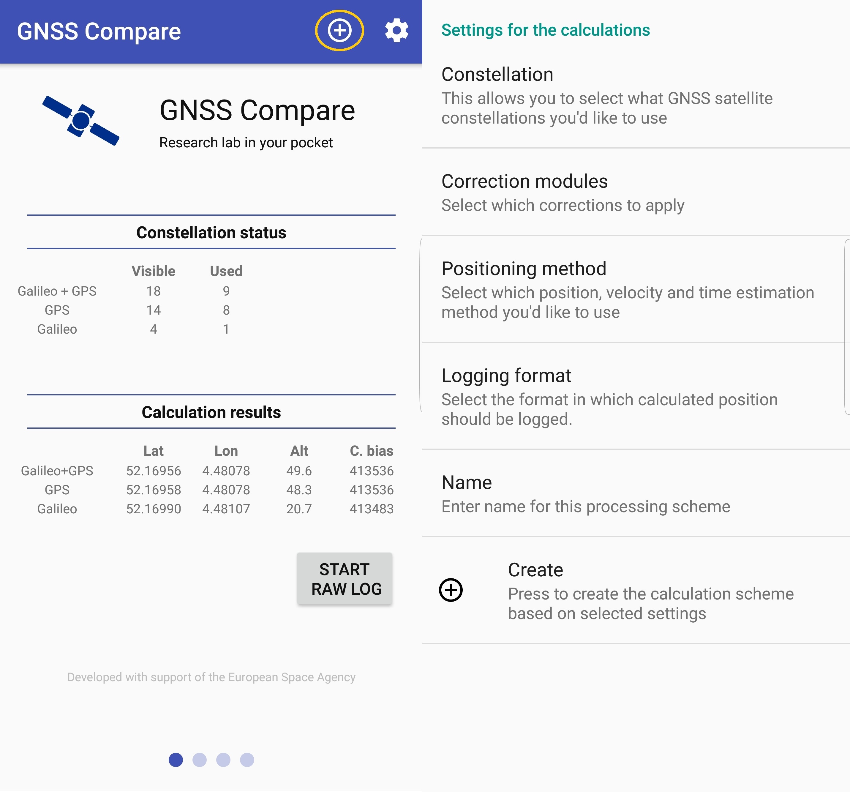
On top there is a blue “stripe” with the name of the application, a “+” and a “gearbox” icon. What are the functionalities of those icons we will see in the Processing schemes part.
Next is the Constellation status header and the information below that shows what GNSS constellations and how many satellites are used to compute PVT. In the GIF above we can see that a combination of Galileo+GPS, GPS only and Galileo only are considered in the algorithms. Moreover, you can notice that not all Visible satellites are being Used in the calculations. The reason behind this is explained in a dedicated chapter of this documentation called Android GNSS raw measurements. Shortly, it is because not all obtained pseudoranges pass a criteria that would allow them to be used in the PVT estimation.
Below the header called Calculation results are the results of the PVT estimators (EKF for this particular example) in terms of: latitude ( Lat ), longitude ( Lon ), altitude ( Alt ) and the receiver’s clock bias ( C.bias ). The UI allows it’s user to make some interesting analysis and to gain some intuitions about the importance of the number of the used satellites in PVT. As example, because there are only 3 Galileo satellites used in the EKF we do expect the estimations of the unknowns to be degraded, which is the case.
And lastly, the START RAW LOG allows the logging of the Android GNSS raw measurements in the exact same format as the Google’s Application GNSS Logger. This feature allows you also to analyze your data in post-processing!
To get to the next view swipe from right to left.
Satellite signal strength
This view is quite straight forward. Here you can monitor the signal strenght of the satellites that are Used in the calculations.
To get to the next view swipe from right to left or to return to the previous one, from left to right.
Positioning error plot
To have an idea of how well the position is estimated, we provide this view that contains a plot with the horizontal position errors using as reference the Android FINE location (i.e., the best location output by the phone). The errors are expressed in meters in the north and east direction (local frame).
Below the plot there is the legend with the specific colors for the chosen processing schemes.
To get to the next view swipe from right to left or to return to the previous one, from left to right.
Google Maps view
In the last view there is the Google Maps on which the position estimations are displayed to be monitored. This can be useful especially when you are testing new PVT algorithms or change the settings of the existing ones (e.g., tunning the EKF). In the GIF below are presented the position estimations by the EKF while the user was in a bus. In this way you can study if your algorithms and their tunning are able to output estimations that follow your dynamics in real-time.
Another useful study that can be made in this view is the comparison of different PVT algorithms. In the example below, one can gain insights about the difference between WLS and EKF. It is interesting to see the performance of an estimator that relies only on measurements relative to an estimator that uses a dynamic model in addition.
To get to the the previous view swipe from left to right.
Processing schemes
By a processing scheme or a calculation module we refer to a set of settings that are considered for the estimation of the smartphone’s position. The user can create a processing scheme in which he/she can choose the following:
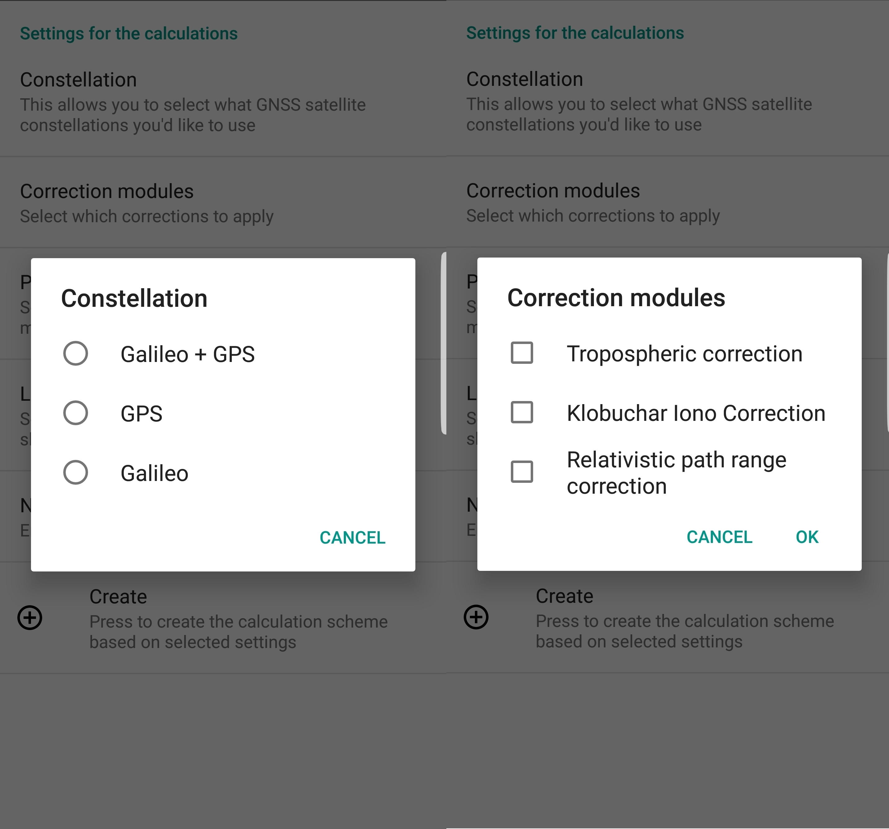
- Constellation: Galileo+GPS, GPS, Galileo
- Correction modules: Tropospheric correction, Klobuchar Iono Correction (only for GPS), Relativistic path range correction
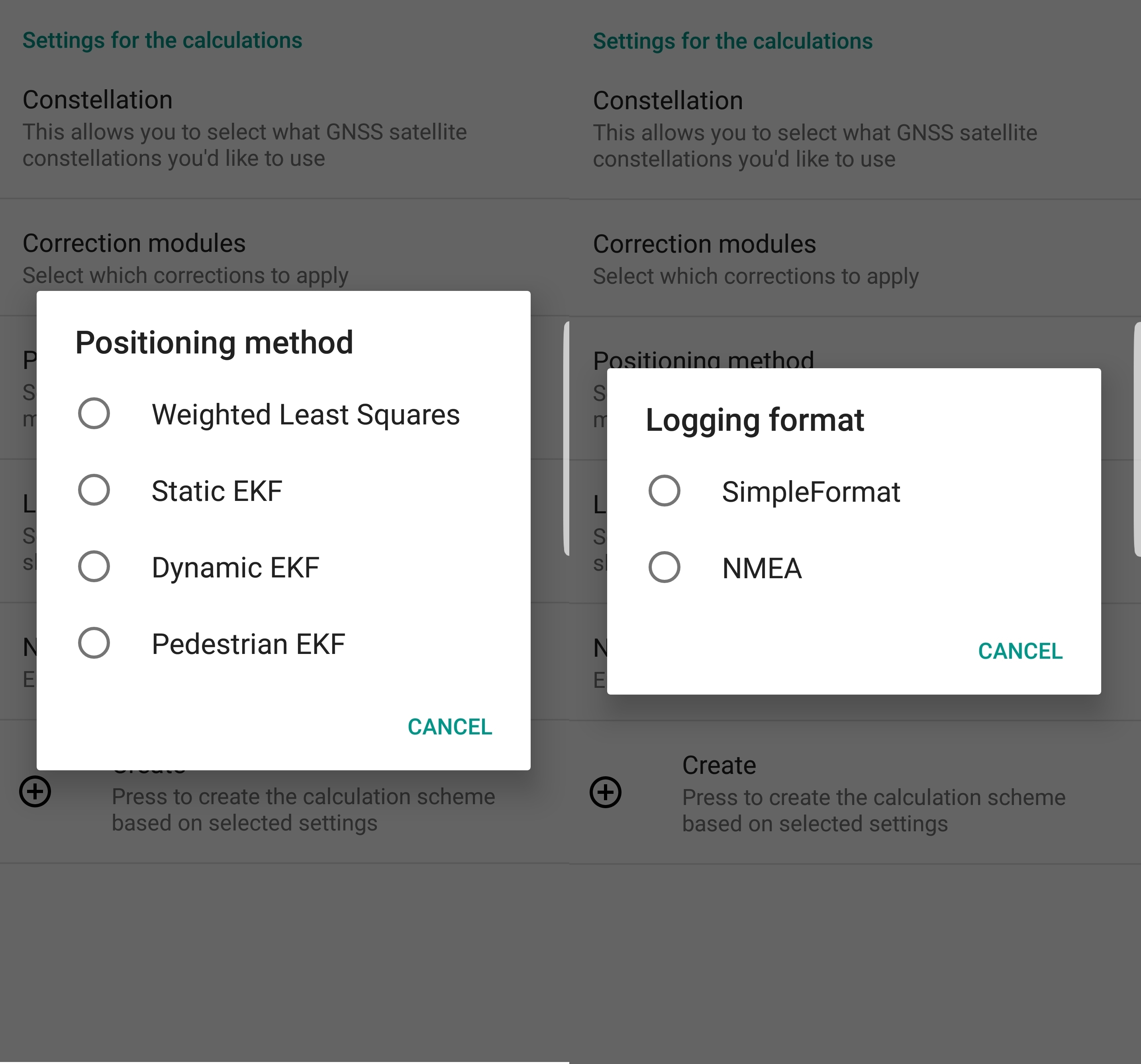
- Positioning method: Weighted Least Squares, Static EKF, Dynamic EKF, Pedestrian EKF
- Logging format: Simple format, NMEA
- Name: The user shall specify the name of the processing scheme
We will continue to show how to create a processing scheme or modify an existing one at the UI level.
Creating a new one
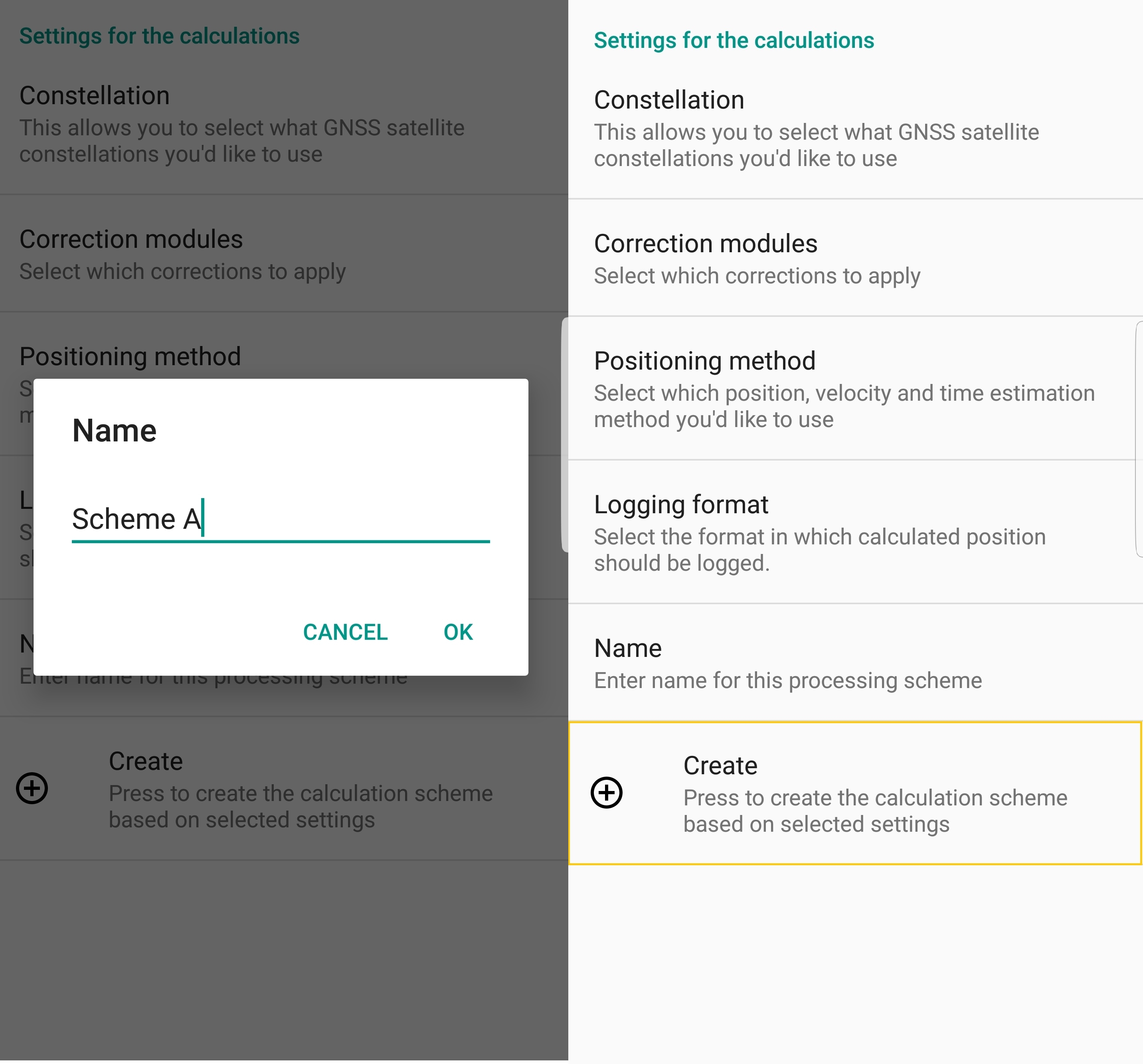
From the Main View select the “+” icon on the top right corner as shown below. A new view will prompt that will allow you to select among the available options.
Let’s begin by selecting the desired Constellation and Correction modules, one at a time.
Next we would like to select the Positioning method and the Logging format.
Finally we have to give a Name to the processing scheme and then press Create.
Modifying an existing one
To modify an existing processing scheme, from the Main View press the “gearbox” icon as shown below.
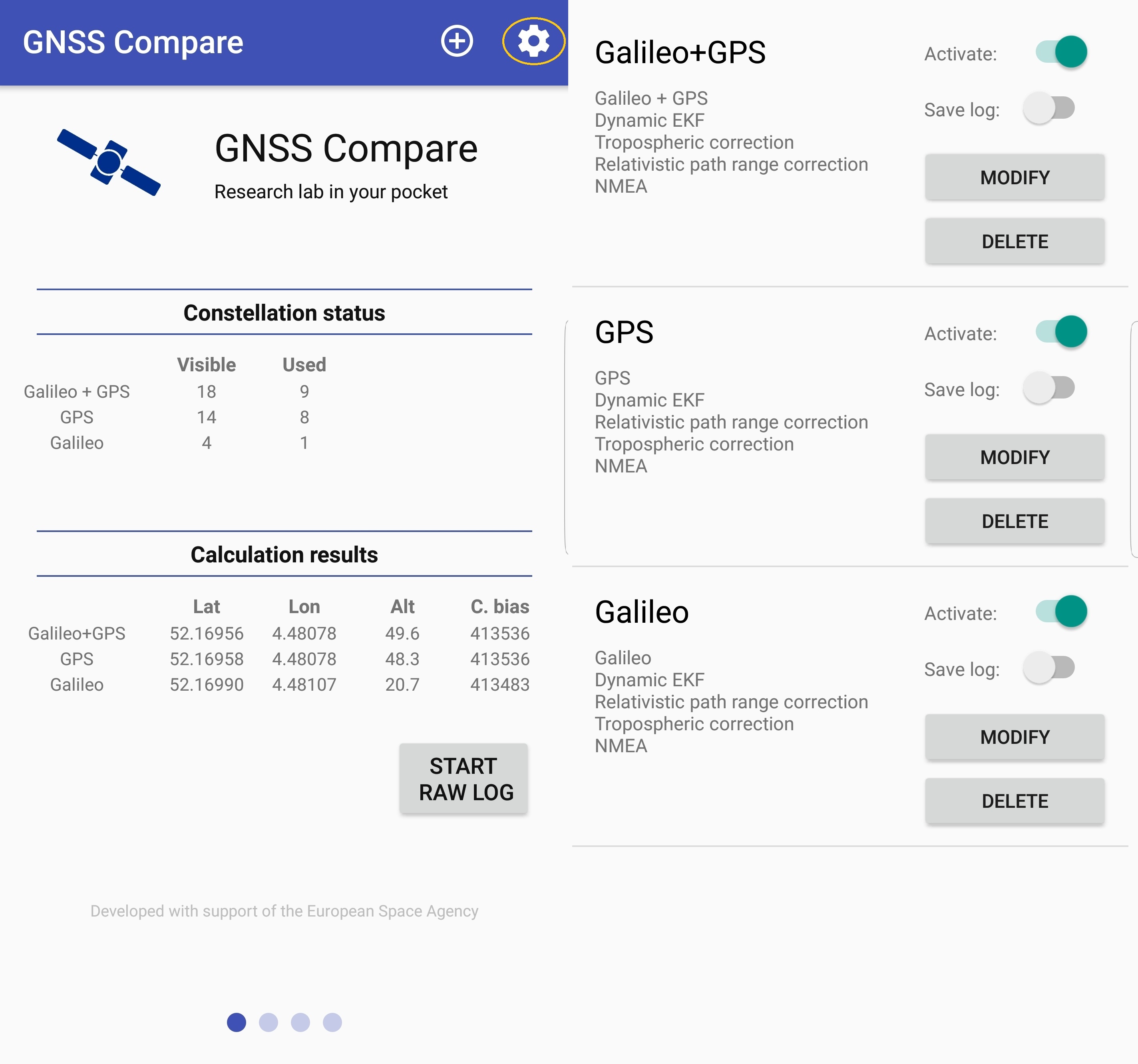
In the right image you can find the created processing schemes. Additionally, there is a summary for each scheme with the chosen options. To change the settings of an existing scheme, press Modify and choose among the existing options. Moreover, in this view you also can enable/disable a processing scheme by pressing the Activate switch or enable/disable data logging with the Save log switch. A dedicated section will be made regarding the logging formats of GNSS Compare.